Rules-text length and lasting Commander popularity in Amonkhet.
Author
firecat1234
Published
September 22, 2026
In the R post, I compared creatures using their printed stats and mana costs. Here, I want to look at the fine print: do wordier Amonkhet cards tend to be more popular years after the set’s release?
The dataset’s EDHREC rank gives us a rough way to explore staying power. Lower ranks mean greater popularity. This is popularity in the saved snapshot, rather than a record of how each card’s popularity changed over time, and it does not measure tournament success. All three comparisons exclude cards marked as reprints in the AKH snapshot, using MTGJSON’s isReprint field. This keeps older cards such as Evolving Wilds out of the analysis.
Read and prepare the cards
import pandas as pdimport matplotlib.pyplot as pltfrom math import log10from statistics import linear_regressionraw_cards = pd.read_csv("data/akh_cards.csv", dtype={"isReprint": "boolean"})raw_cards = raw_cards.loc[~raw_cards["isReprint"]].copy()print(f"Loaded {len(raw_cards)} non-reprint rows from the CSV.")
Loaded 256 non-reprint rows from the CSV.
Some rows are alternate printings, while split cards have separate rows for their two halves. I combine the distinct rules texts for each name before keeping one row per card. Missing text counts as zero words; missing popularity ranks stay missing.
# Keep both halves of split cards without repeating identical printing text.text_by_name = raw_cards.groupby("name")["text"].agg(lambda texts: "\n".join(texts.dropna().unique()))cards = raw_cards.drop_duplicates("name").copy()cards["text"] = cards["name"].map(text_by_name).fillna("")cards["word_count"] = cards["text"].str.split().str.len()cards["edhrecRank"] = pd.to_numeric(cards["edhrecRank"], errors="coerce")# Missing ranks and nonpositive values cannot be used on a logarithmic axis.ranked_cards = cards.loc[cards["edhrecRank"] >0].copy()cards[["name", "rarity", "word_count", "edhrecRank"]].head()
name
rarity
word_count
edhrecRank
0
Angel of Sanctions
mythic
52
8805.0
1
Anointed Procession
rare
21
365.0
2
Anointer Priest
common
44
11410.0
3
Approach of the Second Sun
rare
45
992.0
5
Binding Mummy
common
13
9243.0
How much fine print comes with each rarity?
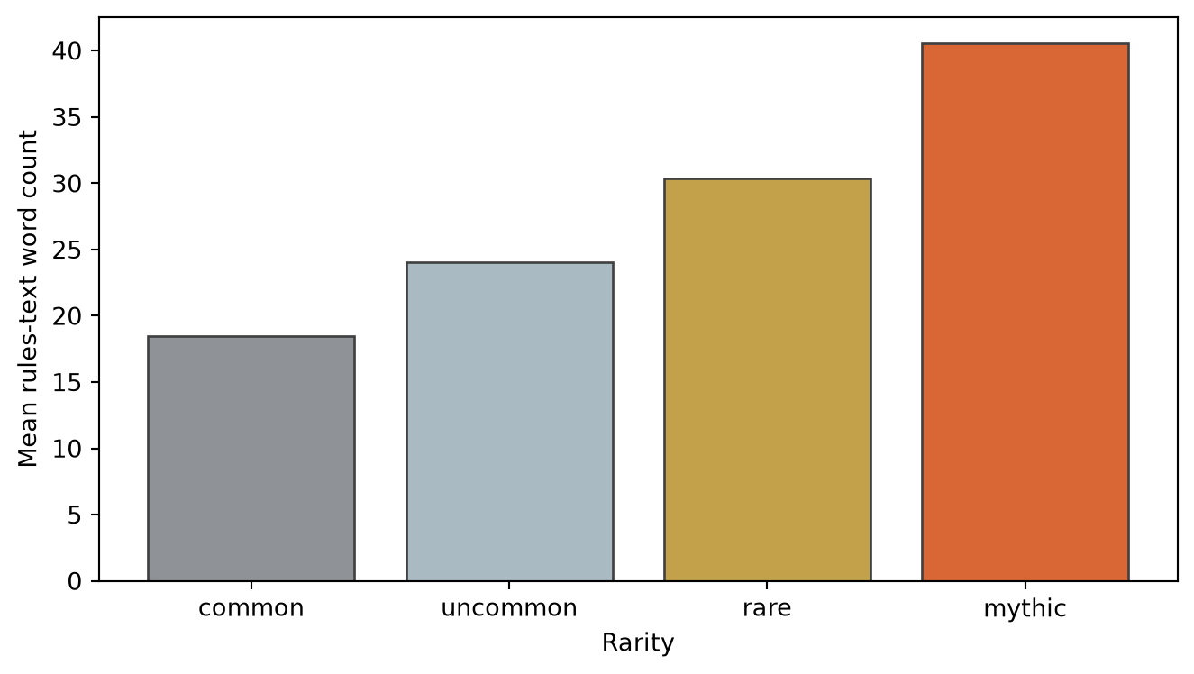
First, I compare average text length by rarity. The word count uses whitespace to split the text, so it includes reminder text and any standalone mana symbols. It is a simple length measure, not a direct measure of how difficult a card is to play. There is a very clear pattern: mean text length increases with rarity.
Figure 1: Mean rules-text word count by rarity for AKH cards not marked as reprints, counting each card once and combining the text of split-card halves.
Does longer text go with greater popularity?
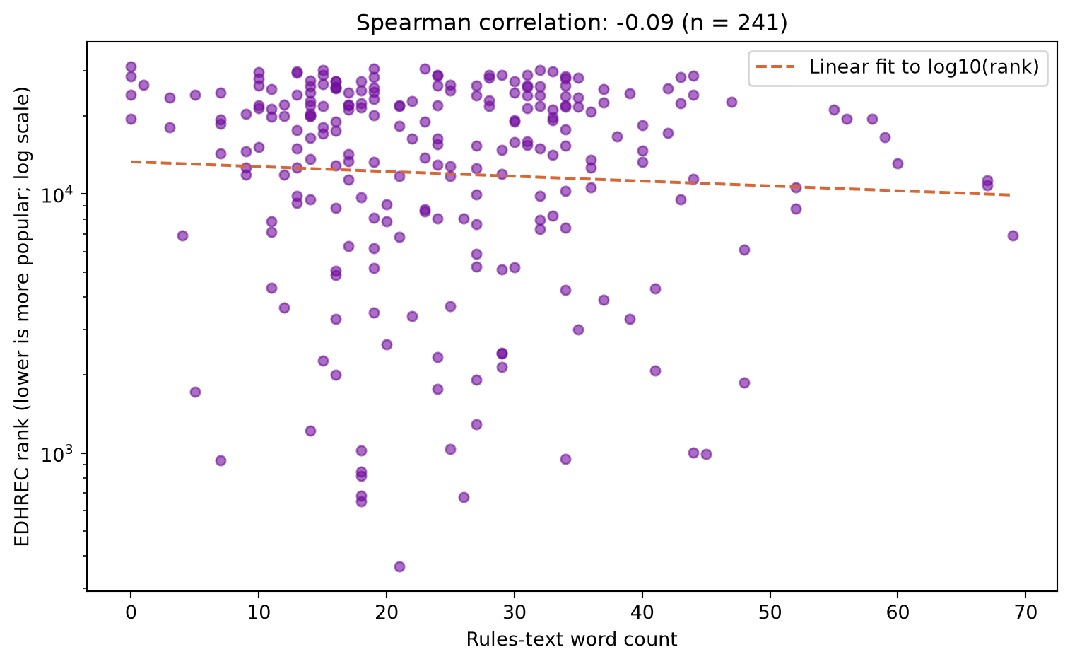
For this comparison, I use only cards with a recorded positive EDHREC rank. The vertical axis uses a logarithmic scale so that ranks across a wide range remain readable. Spearman’s correlation compares the ordering of the two variables: a negative value would mean longer text tends to go with a lower rank, and therefore greater popularity. An association would not establish that longer text causes popularity. That said: there is a low correlation between how wordy a card is and how popular it is now, at ρ = −0.09, so little monotonic association.
# Pearson correlation of the ranks gives Spearman's correlation.# rank() assigns average ranks to ties, so no extra package is needed.rho = ranked_cards["word_count"].rank().corr(ranked_cards["edhrecRank"].rank())# Fit in log-rank space to match the vertical axis.log_ranks = [log10(rank) for rank in ranked_cards["edhrecRank"]]slope, intercept = linear_regression(ranked_cards["word_count"].tolist(), log_ranks)trend_x = [min(ranked_cards["word_count"]), max(ranked_cards["word_count"])]trend_y = [10** (intercept + slope * words) for words in trend_x]fig, ax = plt.subplots(figsize=(8, 5))ax.scatter( ranked_cards["word_count"], ranked_cards["edhrecRank"], color="#720e9d", alpha=0.6, s=25)ax.plot(trend_x, trend_y, color="#D86735", linestyle="--", label="Linear fit to log10(rank)")ax.set_yscale("log")ax.set_xlabel("Rules-text word count")ax.set_ylabel("EDHREC rank (lower is more popular; log scale)")ax.set_title(f"Spearman correlation: {rho:.2f} (n = {len(ranked_cards)})")ax.legend()fig.tight_layout()plt.show()
Figure 2: Rules-text word count versus EDHREC rank for AKH cards not marked as reprints. Lower ranks mean greater popularity; the rank axis is logarithmic. The dashed line is a least-squares fit to log10(rank), separate from the Spearman correlation in the title.
Which cards have stuck around?
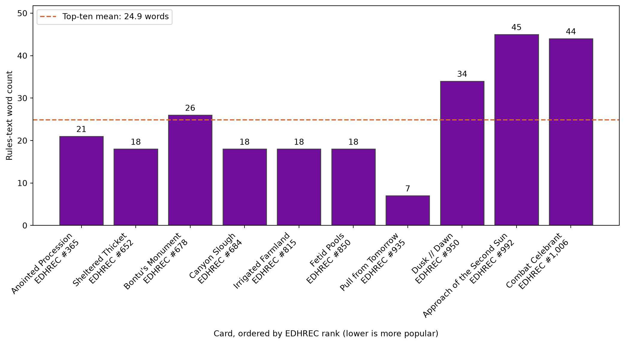
Finally, these are the ten AKH cards with the lowest EDHREC ranks (i.e., most popular) after excluding reprints. Bar height shows rules-text word count, and each card’s label includes its EDHREC rank. The cards are ordered by popularity from left to right, with lower ranks meaning greater popularity.
Figure 3: Rules-text length of the ten most popular AKH cards not marked as reprints. Bars show word counts; the x-axis labels give each card’s EDHREC rank. The dashed line shows the mean word count of these ten cards.
Data: MTGJSON’s Amonkhet dataset, using the saved snapshot dated September 22, 2026, and the CSV prepared in the R post. MTGJSON publishes its data under the MIT licence.
To reproduce the analysis, follow the project README for setup, rendering, and running cells interactively. The data notes explain the CSV format.
AI assistance: ChatGPT helped draft the data preparation and plotting code.